PROJECTS
BITCOIN WALK FORWARD ANALYSIS - Random forest model
PROJECT SUMMARY
This is my first project using machine learning models. I will use the Random forest model on past Bitcoin price data to try to predict if the price of Bitcoin will go up tomorrow by 2%.
I collected the neccessary data from yahoo finance and ran add_all_ta_features on the dataframe to get the the indicators i will need. After that I added custom features reccomended by ChatGPT, set the target, prepared the data for the model and split the target column from the features.
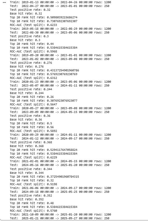
I then created a walk forward analysis using a while loop where I ran the model and collected important data like ROC_AUC score and top 10% hit average.
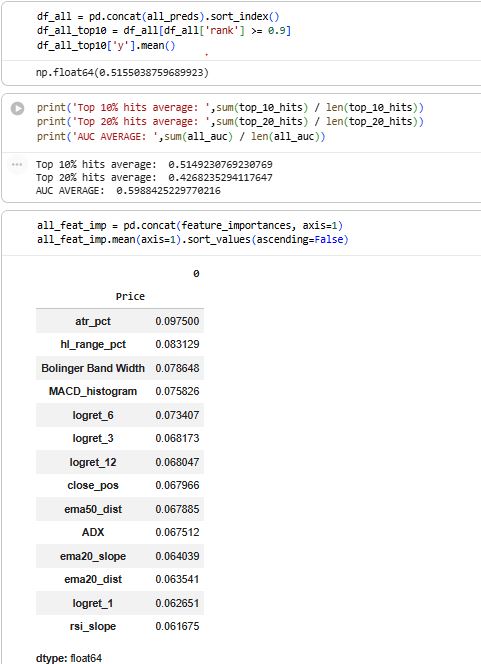
In out-of-sample testing, the model’s highest-confidence 10% of signals achieved a 51.5% hit rate for reaching a +2% move, significantly outperforming the baseline probability.
Github link – https://github.com/Cadez123/BTC_random_forrest_walk_forward_analysis.git
DETAILED DESCRIPTION
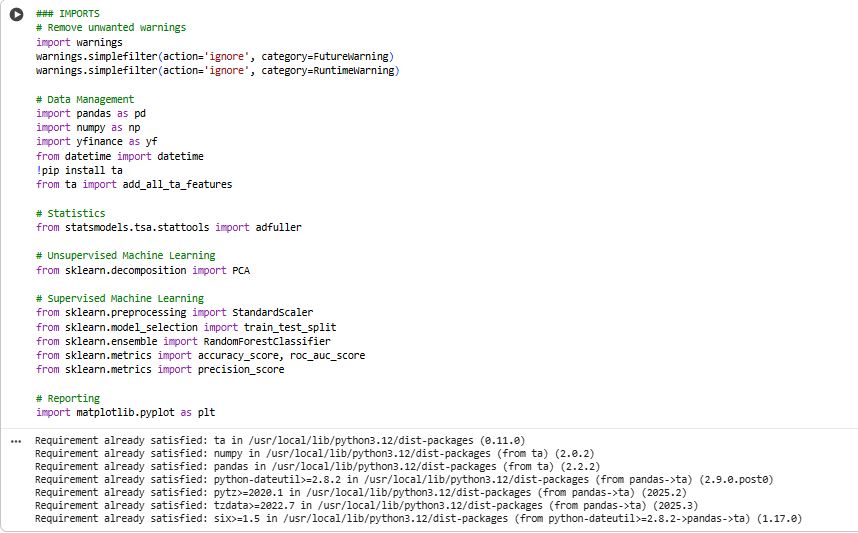
1) Import libraries
Loads Python packages for:
data handling (pandas, numpy)
market data download (yfinance)
technical indicators (ta)
ML + evaluation (scikit-learn)
2) Download daily OHLCV data
Pulls BTC-USD daily candles from Yahoo Finance for a chosen date range.
Creates a clean price DataFrame with Open, High, Low, Close, Volume indexed by date.
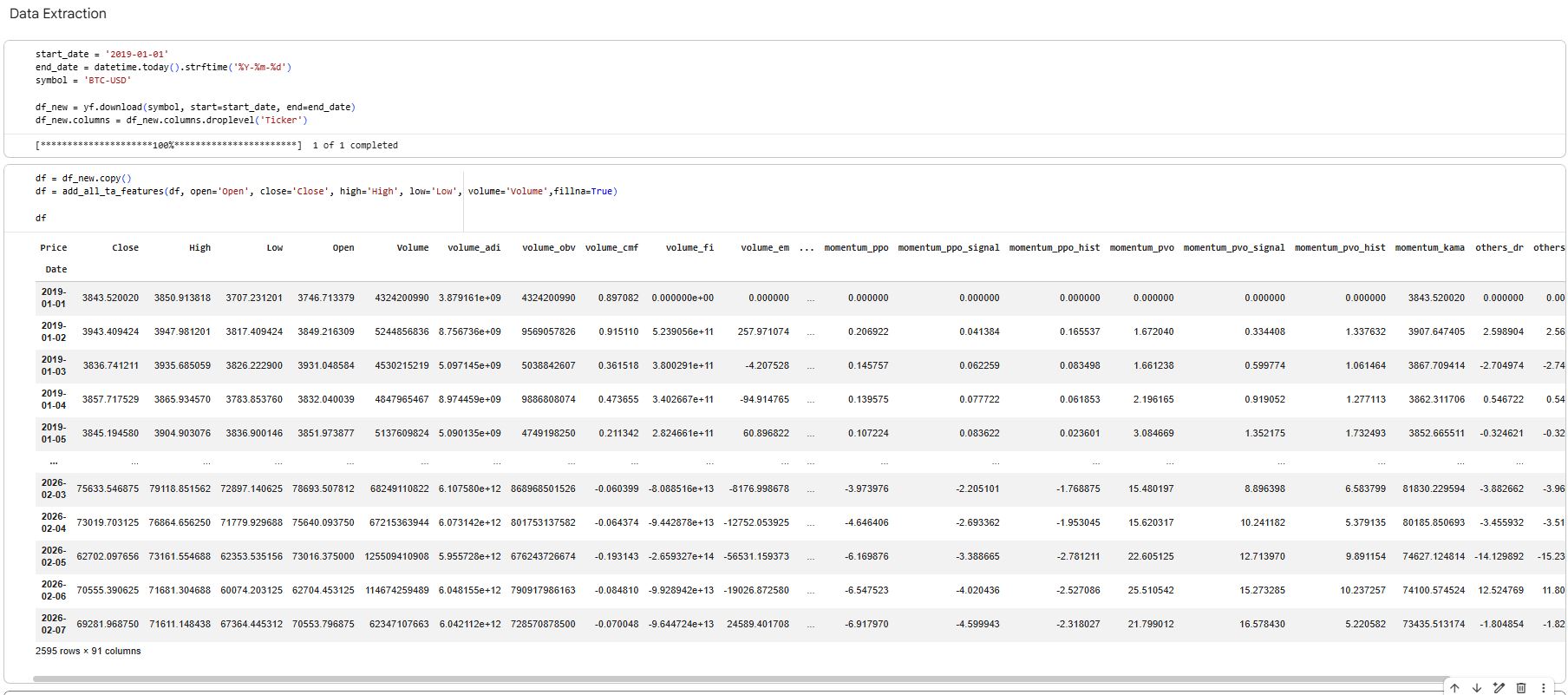
3) Generate technical indicator features
Uses
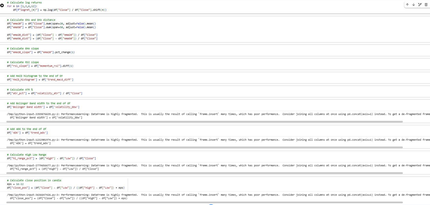
ta.add_all_ta_features(...)to calculate a large indicator set (trend, momentum, volatility, volume-based indicators).Adds extra custom features on top:
log returns over multiple horizons
EMA distance, EMA slope
RSI slope
MACD histogram
ATR %
Bollinger Band width
ADX
candle structure features like high-low range and close position in candle
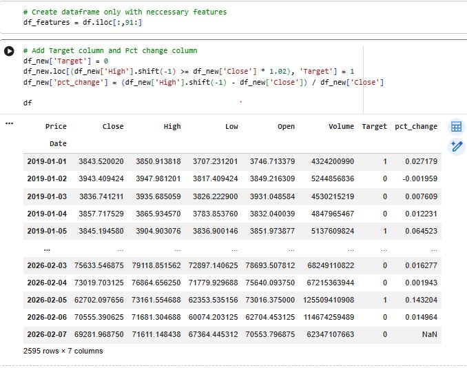
4) Select the feature set
Slices out the final feature block (
df_features = df.iloc[:, 91:]) to keep only the engineered features used for modeling.
5) Create the prediction target
Defines the classification label:
Target = 1 if next day HIGH ≥ today CLOSE × 1.02
else Target = 0
Also computes a helper column (
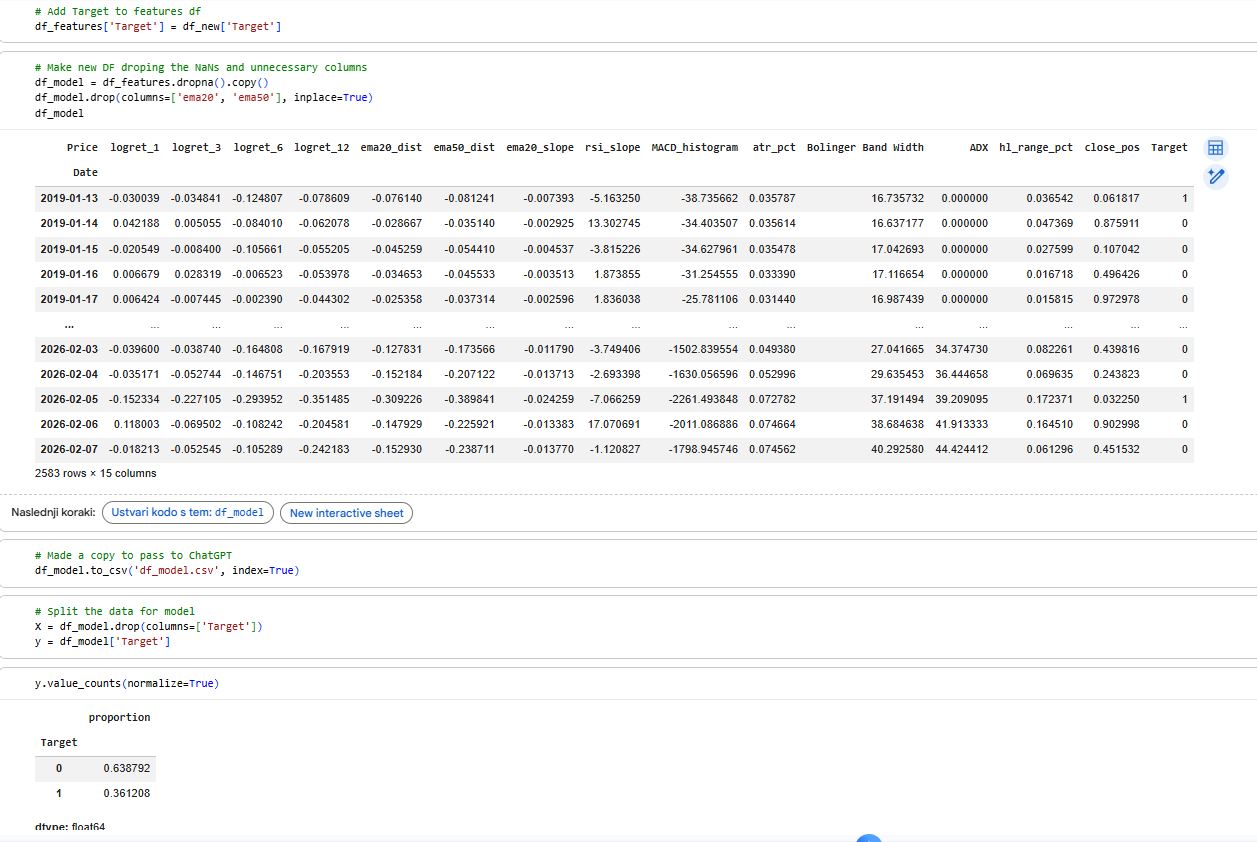
pct_change) to inspect the size of next-day moves.6) Build the modeling dataset
Attaches
Targetto the feature table.Drops NaNs caused by indicator warm-up periods and shifting.
Drops a couple of unused columns (like
ema20,ema50) for the final model table.Exports the final dataset to CSV (
df_model.csv) for reuse/sharing.
7) Split inputs and outputs
Separates:
X= all feature columnsy= the Target column
Runs sanity checks:
same length, aligned index, time-ordered, no missing values
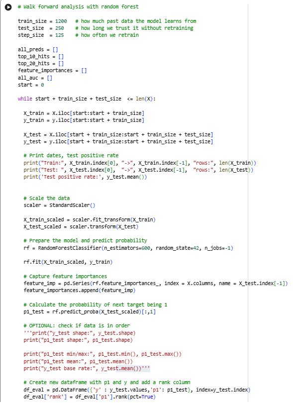
8) Walk-forward training (time-series backtest)
Implements a realistic “train on past → test on future” loop:
Uses rolling windows:
train_size = 1200test_size = 250step_size = 125
For each window:
Split train/test strictly by time (no shuffling)
Fit
StandardScaleronly on training data (prevents leakage)Train a RandomForestClassifier
Predict probabilities (
predict_proba) for the test windowStore results and metrics
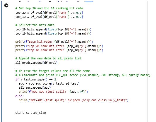
9) Ranking-based evaluation (not fixed thresholds)
For each test window:
Builds
df_evalwith:true label
ypredicted probability
p1
Converts
p1into a percentile rank within that window.Measures how well the model concentrates “wins” in the highest-confidence predictions:
Top 20% hit rate (rank ≥ 0.8)
Top 10% hit rate (rank ≥ 0.9)
10) AUC evaluation per window
Calculates ROC-AUC for each test window (skips windows that contain only one class).
Stores AUCs to later compute the average performance across time.
11) Combine all out-of-sample predictions
Concatenates all window test predictions into
df_all(still out-of-sample only).Computes overall Top-10 performance from
df_all.
12) Feature importance stability across time
Saves
rf.feature_importances_each window.Combines them into a matrix (features × windows).
Computes average importance per feature to see which features stay consistently useful over time.